RESP Charges
Introduction
In CP2K, Restrained Electrostatic Potential (RESP) charges can be fitted for periodic and nonperiodic systems. It is automatically decided by the program whether a periodic or nonperiodic RESP fit is carried out. If the electrostatic (Hartree) potential is periodic (i.e. a periodic Poisson solver is used), a periodic RESP fit is performed. If the Hartree potential is computed using a nonperiodic Poisson solver, the nonperiodic fitting is employed. In any case, a least squares fitting procedure at defined grid points \(\mathbf{r}_k\) is carried out,
where \(V_\mathrm{QM}\) is the quantum mechanical (QM) potential and \(V_\mathrm{RESP}\) the potential generated by the RESP charges. \(N\) is the number of selected fit points.
Nonperiodic fitting
The fitted potential is obtained from a set of point charges \(\{q_a\}\) centered at atom \(a\) according to
For more details see: J. Phys. Chem., 97 , 10269-10280 (1993).
Periodic fitting
The fitted potential is generated from the charge distribution \(\rho\),
where \(g_a\) is a Gaussian function centered at atom \(a\). The periodic fitting is embedded in a Gaussian and plane waves (GPW) framework and described in detail in Phys. Chem. Chem. Phys., 17 , 14307-14316 (2015). In the periodic case, CP2K offers also the possibility to fit the variance of the potential instead of the absolute values, see below.
Basic input
The RESP fitting is a post-SCF step and included as a subsection of the PROPERTIES section.
&PROPERTIES
  &RESP
     &SPHERE_SAMPLING
     &END
  &END RESP
&END PROPERTIES
With this basis setup, the following defaults are employed:
All points outside the van der Waals radii (taken from the Cambridge database) of the atoms are included
The total charge of the system as defined in CHARGE is retained, i.e. INTEGER_TOTAL_CHARGE is set to
.TRUE.by default.All atoms except the hydrogens are weakly restrained to zero, i.e. RESTRAIN_HEAVIES_TO_ZERO is set to
.TRUE.by default.
Sampling of fit points
There are different options to sample the fit points. The fit points can be sampled in shells/spheres around the atoms or, for slab-like systems, in a certain range above the surface. In any case, the systems and the sampled fitting points can be printed as .xyz file and visualized with, e.g. VMD, by enabling:
&RESP
  ....
  &PRINT
    &COORD_FIT_POINTS
    &END
  &END
&END RESP
For better visualization it is recommended to center the coordinates of the systems using CENTER_COORDINATES.
Sphere sampling
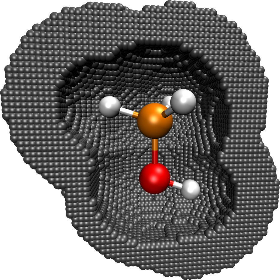
 Figure 1. Methanol molecule and fitting
points (gray) sampled.
This type of sampling is employed for isolated molecules and porous periodic structures suchs as
metal-organic frameworks (MOFs). All grid points within a given spherical shell around the atom are
included in the fitting, see Figure 1. The spherical shells are defined by a minimal radius
\(r_\mathrm{min}\) and a maximal radius \(r_\mathrm{max}\). The paramters \(r_\mathrm{min}\) and
\(r_\mathrm{max}\) can be defined specifically for each element and are, by default, based on the van
der Waals (vdW) radii. For the vdW radii, the values from the Cambridge Structural Database
CAMBRIDGE or the Universal Force Field UFF can be specified via
AUTO_VDW_RADII_TABLE.
Using the keywords
AUTO_RMIN_SCALE and
AUTO_RMAX_SCALE,
\(r_\mathrm{min}\) and \(r_\mathrm{max}\) are then calculated as follows:
\(r_\mathrm{min}\) = AUTO_RMIN_SCALE \(\cdot\) vdW_radius
\(r_\mathrm{max}\) = AUTO_RMAX_SCALE \(\cdot\) vdW_radius
These settings can be overwritten for all atoms using the keywords RMIN and RMAX or only for specific atoms using RMIN_KIND and RMAX_KIND. In the following example, \(r_\mathrm{min}\) is overwritten for all carbon atoms to 2.1\(\,\mathring{\mathrm{A}}\).
&SPHERE_SAMPLING
  AUTO_VDW_RADII_TABLE CAMBRIDGE
  AUTO_RMIN_SCALE 1.0
  AUTO_RMAX_SCALE 10.0
  RMIN_KIND 2.1 C
&END
Slab sampling
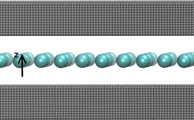
RESP charges can be also fitted for slab-like systems. In this case, the potential should be well reproduced above the surface where, e.g., adsorption processes take place. The input for a flat monolayer, see Figure 2, is for example:
 Figure 2. Flat monolayer and fitting
points (gray).
&SLAB_SAMPLING
  RANGE 1.0 3.0
  ATOM_LIST 1..32
  SURF_DIRECTION Z
&END
&SLAB_SAMPLING
  RANGE 1.0 3.0
  ATOM_LIST 1..32
  SURF_DIRECTION -Z
&END
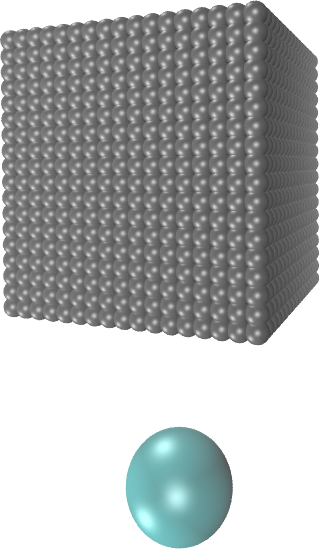
 Figure 3. Fit points sampled over
surface atom.
Here, the system is 2D-periodic in the xy-dimensions and the fitting points are sampled above (+z-direction) and below (-z-direction) which is specified by SURF_DIRECTION. With the keyword ATOM_LIST the atoms that constitute the surface are defined. This list should contain indexes of atoms of the first surface layer. RANGE defines that the points are sampled between 1-3 \(\mathring{\mathrm{A}}\) above the surface layer.
The sampling technique is flexible enough to follow a corrugation of the surface. The sampling technique works as follows: An orthogonal box with box length \(abc\) is constructed over each surface atom, see Figure 3. All fitting points within this box are included in the fitting. The height \(c\) of the box is defined by the keyword RANGE . The length \(a=b\) are given by the keyword LENGTH. For flat surface layers, LENGTH is set to a sufficiently large values (3 \(\mathring{\mathrm{A}}\) or more). For corrugated surface layers, LENGTH should be in the range of the distance between the surface atoms.
An input example for a corrugated graphene layer on ruthenium, see Figure 4, is given below. ATOM_LIST lists in this case the indexes of the carbon atoms.
 Figure 4. Corrugated graphene layer
on ruthenium and fitting points (gray).
&SLAB_SAMPLING
  RANGE 2.0 4.0
  LENGTH 2.0
  ATOM_LIST 1..1250
  SURF_DIRECTION Z
&END
Constraints
A constraint on the total charge of the system is introduced by the keyword
INTEGER_TOTAL_CHARGE, which is set by
default to .TRUE.. Further explicit constraints can be given via the subsection
CONSTRAINT. It is possible to enforce the same
charges for chemically equivalent atoms, e.g. for the hydrogen atoms of a methyl group. The
corresponding input is:
&CONSTRAINT
  EQUAL_CHARGES
  ATOM_LIST 1 2 3
&END
where ATOM_LIST lists the indexes of the atoms that should have the same charge.
The definition of more elaborate constraints is also possible. The constraints are always linear following the formula \(\sum_i^{N_\text{list}}c_i q_i=t\). The sum is running over the atoms given in ATOM_LIST and \(t\) is the target value of the constraint given by TARGET. The coefficients \(\{c_i\}\) are defined by the keyword ATOM_COEF. With the following input it is achieved that the (absolute value) of the charge on atom 3 is twice as large as the charge on atom 5, i.e. \(q_3=2q_5\).
&CONSTRAINT
  ATOM_LIST 3 5
  ATOM_COEF 1.0 -2.0
  TARGET 0.0
&END
Restraints
To avoid unphysical values for the fitted charges, restraints can be set. The restraints in CP2K are addressed by harmonic penalty functions,
where \(t_j\) is the target value for charge \(q_j\) and \(\beta\) is the strength of the restraint. By
default, all elements except hydrogen are weakly restrained to zero, i.e. the keyword
RESTRAIN_HEAVIES_TO_ZERO is set
to .TRUE. by default. The strength of this restraint is controlled by
RESTRAIN_HEAVIES_STRENGTH.
Restraints can be also defined explicitly via the subsection
RESTRAINT:
&RESP
  ...
  &RESTRAINT
    ATOM_LIST 1..3
    TARGET -0.18
    STRENGTH 0.0001
  &END
  &RESTRAINT
    ATOM_LIST 4
    TARGET 0.21
    STRENGTH 0.0001
  &END
  RESTRAIN_HEAVIES_TO_ZERO .FALSE.
&END RESP
In this example, charges on atoms with indexes 1..3 are restrained to -0.18 and the charge on atom 4
to 0.21. The target values \(t_j\) of the restraints can be, e.g., inspired from DDAPC, Mulliken
charges etc. The strength \(\beta\) of the restraint is defined by
STRENGTH. Large values for \(\beta\) will
limit increasingly the flexibility of the charge fitting and decrease the quality of the fit. If
only the explicitly given restraints should be used,
RESTRAIN_HEAVIES_TO_ZERO must be
switched to .FALSE..
Fitting the variance (REPEAT method)
CP2K offers also the possibility to fit the variance of the potential as proposed in Campana2009. This is only valid for periodic systems, since the reference state of the ESP is arbitrary in the periodic case. The modified residual reads:
where
When \(V_\mathrm{QM}\) is obtained from, e.g., a plane wave code and the periodicity of \(V_\mathrm{RESP}\) is later treated by, e.g., Ewald summation, both potentials will have different offsets. The modified residual \(R_\mathrm{repeat}\) was introduced to overcome this problem. In CP2k, \(V_\mathrm{QM}\) and \(V_\mathrm{RESP}\) are both evaluated with the same method, the GPW approach, and have thus the same offset. However, fitting the variance of the potential is an easier task than fitting the absolute values and avoids a strong fluctuation of the charges. A stabilization of the fitting procedure is thus also expected in CP2K when \(\delta \ne 0\). The value of \(\delta\) depends on the sampling of fitting points. If all points are included, it strictly holds that \(\delta=0\), since we have \(\sum_k^{N_{all}}V(r_k)=0\) (in CP2K). In this case, the original and modified residuals are identical, i.e. \(R_\mathrm{esp}=R_\mathrm{repeat}\). If the fitting points are sampled in spheres around the atom, which is done for molecular periodic structures like MOFs, \(\delta\) will be non-zero and fitting the variance is strongly recommended. When sampling the fitting points above a surface, we often find that \(\delta\sim0\). However, minimizing \(R_\mathrm{repeat}\) will partly also yield improvements for such systems.
To enable this option, add the keyword USE_REPEAT_METHOD:
&RESP
  ...
  USE_REPEAT_METHOD
&END RESP
Note that
RESTRAIN_HEAVIES_TO_ZERO is then
automatically switched to .FALSE.. Furthermore, the definition of explicit restraints is usually
not necessary.
To obtain REPEAT charges in a stricter sense, i.e. as computed by the REPEAT code, sphere sampling has to be enabled, the van der Waals radii must be retrieved from the Universal Force Field and the total charge must be retained. The corresponding input is
&RESP
  USE_REPEAT_METHOD
  &SPHERE_SAMPLING
     AUTO_VDW_RADII_TABLE UFF
   &END
&END RESP
Use the keyword AUTO_RMIN_SCALE and AUTO_RMAX_SCALE to scale the van der Waals radii as described above. Note that small numerical deviations compared to the REPEAT code are possible since the fitting is embedded in a GPW framwork as described in Phys. Chem. Chem. Phys., 17 , 14307-14316 (2015) , whereas the REPEAT code uses Ewald summation.
Check the quality of the fit
A measure for the quality of the fit are the root-mean square (RMS) error
and the relative root-mean square (RRMS) error
Both errors are printed to the output file. They should be as small as possible. Typical values can be found here:
When the variance is fitted, \(V_\mathrm{RESP}\) is shifted by \(\delta\) with respect to \(V_\mathrm{QM}\). Thus, \(V_\mathrm{RESP}\) is replaced by \(\tilde{V}_\mathrm{RESP}=V_\mathrm{RESP}+\delta\) in the formulas for the RMS and RRMS values.
The RESP potential can be printed in cube file format using the following option:
&RESP
  ....
  &PRINT
    &V_RESP_CUBE
    &END
  &END
&END RESP
The QM potential can be as well printed as cube file using V_HARTREE_CUBE. The cube files can be visualized with, e.g. VMD, and the RESP and the QM potential can be directly compared. Note that \(\tilde{V}_\mathrm{RESP}\) is printed instead of \(V_\mathrm{RESP}\) when the variance is fitted.
Example input files
Isolated methanol molecule - nonperiodic fit: methanol_nonperiodic
Metal-organic framework IRMOF-1 - periodic fit using REPEAT: irmof-1_REPEAT
Metal-organic framework MIL-53-Al - periodic fit using REPEAT: mil-53-al-repeat
Graphene on Ru(0001) - periodic fit: graphene_Ru